OBJECTIVES:
INTRODUCTION:
In all these examples one discovers that, if one repeats the observation,
the new number will differ from the preceding one. More
importantly the number found can not be predicted using the knowledge of a
preceding observation nor can it be used to predict the following one.
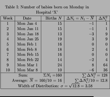
For example the number of babies born
on a particular Monday will usually be different from the number born on the
succeeding Monday. Similarly, the number of patients (out of a different
one thousand) that feel better after taking
a particular kind of pain reliever, or the number of murders in the
following year in New York City will be unpredictably different.
![$\textstyle \parbox{0.46\linewidth}{
\includegraphics[height=4.8cm]{figs/l104/fnc1a-1.eps} \\
Fig. 1: Distribution of Monday births
}$](img474.png)
What does the figure tell you?
![\includegraphics[height=6.cm]{figs/l104/fnc1a-2.eps}](img477.png)
You may argue that the value of ![]() in the two examples was obtained using
many observations; how can one know its value if one does only one
observation?
in the two examples was obtained using
many observations; how can one know its value if one does only one
observation?
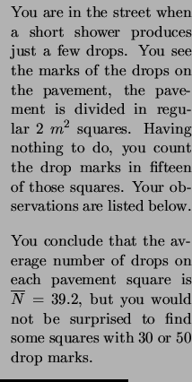
In other words, if I make only one observation, for instance if I
find that the number of drops
in a single square is ![]() , what can I say about how far from the unknown
but true value
, what can I say about how far from the unknown
but true value ![]() it is likely to be?
it is likely to be?
REQUIRED KNOWLEDGE:
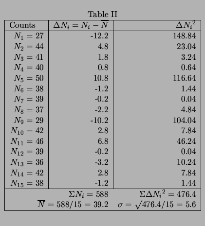
If one makes a histogram of the number of times a certain count appears one
finds a bell shaped curve called a ``Gaussian distribution'' centered on
the average.
The histogram below looks a lot better than the ones you have seen above;
this is so because it shows the distribution of many more observations.
![\includegraphics[height=6.5cm]{figs/l104/fnc1a-3.eps}](img482.png)
The histogram shows that counts of about 100 are most frequent, and that counts of 70, or 130 are much less likely to occur; we can think of the ``width'' of the curve i.e. the range of the counts that occur most frequently is about 20.
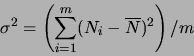
Statistical theory predicts that the width of the curve, the
``standard deviation'' of the distribution is defined as:
The standard deviation ![]() is a measure of how wide the curve is;
about 1/3
of the counts will lie outside the interval
is a measure of how wide the curve is;
about 1/3
of the counts will lie outside the interval
![]() to
to
![]() .
.
Only about 1/20
of the counts will lie outside the interval
![]() to
to
![]() .
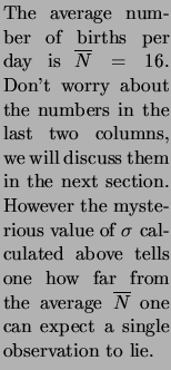
The value of
.
The value of ![]() is calculated automatically by your computer, so you do
not really have to worry about it.
However here goes the formula, you may skip this if you
wish.
is calculated automatically by your computer, so you do
not really have to worry about it.
However here goes the formula, you may skip this if you
wish.
EXPERIMENT
Instead of collecting data from the hospital, from the department
of transportation or the NYPD, of the kind shown in the examples above, we will
make our own homemade random distribution using the random decay of
long lived radioactive nuclei.
You will study the statistics of counting.
You will find how the precision with which one can measure
a decay rate R depends on the total number of counts, which in this case
is proportional to the time interval during which you observe the radiation.
The rate ![]() of the disintegration of the Radioactive sample
is obtained by allowing the G-M counter to detect the radiation emitted for
a length of time
of the disintegration of the Radioactive sample
is obtained by allowing the G-M counter to detect the radiation emitted for
a length of time ![]() , and dividing the number
, and dividing the number ![]() of observed counts by the
time:
of observed counts by the
time: ![]() .
.
If you were to repeat the experiment, for the same time interval ![]() , the number
of counts would almost certainly not be the same because of the random
nature of radioactive decay. How accurately would you then know the
real value of the rate?
Intuition tells you that a rate measured with a long time interval
, the number
of counts would almost certainly not be the same because of the random
nature of radioactive decay. How accurately would you then know the
real value of the rate?
Intuition tells you that a rate measured with a long time interval ![]() is
going to be more reliable than one taken with a short time interval.
But
even so just how reliable would either of these be? A better way to
ask this question is:
is
going to be more reliable than one taken with a short time interval.
But
even so just how reliable would either of these be? A better way to
ask this question is:
If I repeat the experiment, and obtain a different
new rate, how big, on the
average do I expect the difference between the two rates to be?
EQUIPMENT
![\includegraphics[height=5.2cm]{figs/l104/fnc1a-4.eps}](img494.png)

| PRECAUTIONS:
The Geiger counter has a very thin window to permit the entry of |
PROCEDURE I:
|
|
|
 |
||
| mean | std. dev. | rel. unc. | ||
and enter it in column 5 of the table.
versus
QUESTIONS