HC-1  The Ideal Gas Law and Absolute Zero

OBJECTIVES:

To observe the behavior of an ``ideal'' gas (air) and to determine absolute zero (in Celsius).

FUNDAMENTAL CONCEPTS:

The behavior of an ideal gas under varying conditions of pressure and temperature is described by the ``Ideal Gas Law'':

$$PV = nRT \eqno(1)$$

Where $P$ is the pressure (in Pascals, $Pa$), $V$ is the volume (in $m^3$), $T$ is the temperature in Kelvins (K= C$+ 273$), $n$ is the number of moles present (1 mole $\equiv 6.023 \times 10^{23}$), and $R$ is the gas constant ( $8.31 J/mol \cdot K$).
This equation is a combination of two laws which were discovered previously:

1. Boyle's Law relates volume and pressure of a fixed quantity of gas at a constant temperature: $PV = constant$
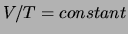
2. Charles' Law relates volume and temperature of a fixed quantity of gas at a constant pressure $V/T = constant$

Gay-Lussac finally combined the two laws into the ideal gas law shown in Eqn. 1.
In EXPT. I Boyle's law will be verified by varying $V$ and $P$ (assuming fixed $T$).
In EXPT. II You will vary $T$ and $V$ to determine the value of absolute zero.

APPARATUS:

Basic equipment: EXPT. I - Lab stand; 60 cm$^3$ plastic syringe attached to a plastic ``quick-connect'' coupling.
EXPT. II - PASCO Steam generator; water jacket container; steel Dewar flask; small stainless steel can with a volume of $98$ cm$^3$ with a ``quick release'' connector; FLUKE digital thermometer and temperature probe

Computer equipment: Personal computer set to the HC1 lab manual web-page; PASCO interface module; PASCO pressure sensor (mounted on lab stand).

EXPERIMENT I: BOYLE'S LAW

1. CLICK on the telescope icon below to initiate the PASCO $^{\mbox{\copyright}}$ interface software. The computer, monitor and PASCO interface must already be on and pressure sensor plugged into the A DIN connector position. (If not see your instructor.)

2. The PASCO software window should display graphs configured to display pressure $vs$ volume and pressure $vs$ inverse volume, a table for these three values, a panel meter for the instantaneous pressure reading.
   Since there is no automated volume measurement you will have to enter these data points manually.
   NOTE: The volume is recorded in milliliters (1 mL = 1 cm$^3$) and the pressure in kilopascals ($kPa$). In this case the ideal gas law ($PV=nRT$, $T$ in Kelvin) uses $R = 8.31 \times 10^3$(kPa$\cdot$cm$^3$)/(mol$\cdot$K).

3. If the syringe is attached to the pressure sensor, disconnect it at the twist-lock quick connect coupling. Set the syringe plunger to the 60 cm$^3$ mark and then reconnect it to the pressure sensor. Make sure that the equipment looks as sketched in Fig. 1.

   Figure 1: Sketch of pressure sensor and syringe/plunger assembly.

   

4. Initiate the data acquisition by clicking on the REC button in the upper left panel. A large window for keyboard entry will appear (i.e. Keyboard Sampling). There is no automated volume measurement for the plunger position so you will use the keyboard to enter data points manually.
   Slowly push the plunger in to the 50 cm$^3$ position (about 10 seconds) and back to the original setting while watching the panel pressure meter and record in your lab-book the readout precision of the pressure sensor.

5. Now begin the actual data logging by clicking the mouse on the numeric entry field in the Keyboard Sampling window, replacing the current value with 60.0 and then striking the Enter key. Data logging should be confirmed by observing a new data point on the plots and three new values in first row of the table. The PASCO software will try to anticipate your next volume setting in the Keyboard Sampling window. You should change this value to the appropriate value before logging your next data point.

6. Reduce the volume slowly in discrete 5 cm$^3$ increments while logging the data at each step (see the previous item) until you reach 20 cm$^3$. Then as a check, slowly increase the volume in 5 or 10 cm$^3$ steps (remember to log the data) until you reach 60 cm$^3$.

7. Stop the data acquisition and transfer your data to a table in your write-up and comment on the reproducibility of your measurements. Do your plots have the correct functional behavior? Your can refrain from printing out the graphs until your have performed a linear regression using either the PASCO graphical analysis capabilities or the Vernier GA graphical analysis package.

8. Which of the two graphs do you expect to be a straight line and why? For this ``curve'' what is the expected $y$ intercept? Now fit this data to a line (using linear regression) and record the slope and intercepts with the appropriate units. Print out the respective plots and include them in your lab write-up.

9. OPTIONAL: Repeat the procedure of item 4 except move from 60 to 20 cm$^3$ as rapidly as possible and record the pressure data at the start and stop points. Are the pressure readings consistent with those of the ``slow'' moving experiment? If not can you suggest a reason?

QUESTIONS:

I.

Does the line go through the origin as expected? By how much should you change the pressure readings so that the line goes through the origin?

II.

What are the possible sources of error in this experiment? For each source, try to decide what effect it might have on the experimental results.

III.

Read the barometer that is located in your laboratory room, ask your instructor for help if you are having trouble. Convert the pressure from cm of Hg to $kPa$ and compare this value with the one obtained at 60 cm$^3$ in step 5. Is the difference between the two readings important? Does it affect your conclusions?

IV.

OPTIONAL: Assuming that there are 22.4 liters per mole of an ideal gas, how well does your observed slope agree with your expected slope?

EXPERIMENT II: IDEAL GAS LAW

In this part the Ideal Gas Law is verified by observing the pressure of a fixed volume of gas at four different temperatures: Room temperature, 100 $^o$C, 0 $^o$C and -197 $^o$C. Since $PV=nRT$ and $T=T_{\mbox{\tiny Celsius}}+T_0$ we can rewrite this as

$$P(T_c) = \frac{nR}{V} T_c + \frac{nR}{V} T_0$$

and thereby determine the value of absolute zero ($T_0$) from the intercept.

SUGGESTED PROCEDURE:

1. CLICK on the telescope icon below to initiate the PASCO $^{\mbox{\copyright}}$ interface software. The computer, monitor and PASCO interface must already be on and pressure sensor plugged into the A DIN connector position. (If not see your instructor.)

2. Attach the small stainless steel can (volume of $98$ cm$^3$) as shown below to the PASCO pressure sensor using the plastic ``quick release'' connector. Raise the assembly up if necessary. Turn on the Fluke thermometer. Unless the stainless steel can has been recently used it should now be at room temperature.

   Figure 2: Sketch of pressure sensor and stainless-steel can assembly.

   
   
   

3. Initiate the data acquisition by clicking on the REC button. There should be a single plot (temperature vs pressure), a panel meter for pressure and a keyboard entry window. Record the Fluke meter reading in the keyboard entry window (if uncertain see EXPT. I, item 5 for a more complete description). Pause the data acquisition by clicking on the PAUSE button.

4. Fill the PASCO steam generator with water and turn it on. The level of the water should be $\sim 3 cm$ below the top, or about 1/2 - 3/4 full (Fig. 3). Turn the knob to 9 until the water boils and then turn it down somewhat.

   Figure 3: PASCO steam generator.

   

   
   

5. As soon as the water in the steamer is boiling, raise the pressure sensor stand and then lower it so as to immerse the stainless steel can in the boiling water.

6. Wait until the water is boiling again and then put the Fluke thermometer in the boiling water. Resume the data acquisition by clicking on the REC button. Watch the pressure readout and after it is stable (with time) record the Fluke temperature in the data entry window. Turn the PASCO steam generator off and remove the small stainless steel can from the bath. Pause the data acquisition.

7. Fill the water jacket container with water and ice. The level of the water should be $\sim 5 cm$ below the top. Repeat the last two steps for obtaining the 0 $^o$C pressure reading. Empty and dry the stainless steel dewar.

8. Take the stainless steel dewar and ask the instructor to fill your dewar with liquid Nitrogen and repeat step 3 for the container at liquid Nitrogen temperature.

9. Stop the data acquisition and transfer your data to a table in your write-up. Do your plot have the correct functional behavior? Your can refrain from printing out the data until your have performed a linear regression using either the PASCO graphical analysis capabilities or the Vernier GA analysis package.

10. For your curve what is the expected $y$ intercept? Now fit this data to a line (using linear regression) and record the slope and intercepts with the appropriate units. Print out the plot and include it in your lab write-up.

QUESTIONS

I.

What is the percentage difference between the value you found and the accepted value for absolute zero?

II.

Assuming that ice water is exactly at 0 $^o$C and the boiling water is at 100 $^o$C, estimate the systematic error introduced into your absolute zero measurement? Does this improve your results?

III.

OPTIONAL: Qualitivity what error results from the gas in the small tube not being always at the can temperature?

IV.

OPTIONAL: Does thermal expansion of the can affect your results? In what way?